But the recurrence does, for large parameter, generate a chaotic sequence which has useful analogies to waether, climate and their emulation. Here is a plot of part of that sequence. The green, red and blue points are initially separated by a distance of 0.0001 K. The recurrence starts at T0=300K, and follows the sequence
Tn+1=Tn+b*(1-(Tn/Te)4) Te=243K, b=170
I follow three sequences, red starting at T0=300K (red), with green and blue separated there from red by 0.0001 K.
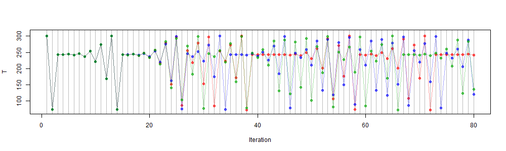
They are initially indistinguishable, but start to separate after about 25 iterations, and although they then sometimes come together, after about 50 timeteps there is really no association between them. You can't usefully predict where any starting point will lead to at that time, because the differences in those initial values are unlikely to be measurable. In fact, as I indicated in the last post, the growth in separation is initially exponential, so the slightest difference in floating value, say 1e-12, will lead to separation delayed by only another thirty or so iterations. I'll give much more detail about this process below.
Weather forecasting is similar. An initial state can be measured with finite accuracy, but small discrepancies grow, so the calculated forecast is useful for only about ten days at most. There is every reason to believe that the Earth itself has a corresponding magnification of small changes. So a perfect emulator could still not predict.
However, some things can be said. The plot remains within finite bounds, the same for each color. You can see that there are patterns whereby sequences of temperature around T0 are frequent. I will show histograms of frequency of temperatures, which are strongly patterned, and the same for each trajectory. These are the "climate", which is what can be determined in the presence of chaos. And they apply independent of starting points. Finding them is a boundary value problem, not an initial value problem.
I will also show that the climate is quite dependent on the parameter b, and that its dependence can be reliably determined from solution sequences, analogous to GCM runs.
The "climate" of chaos
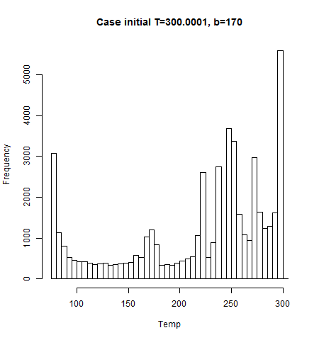
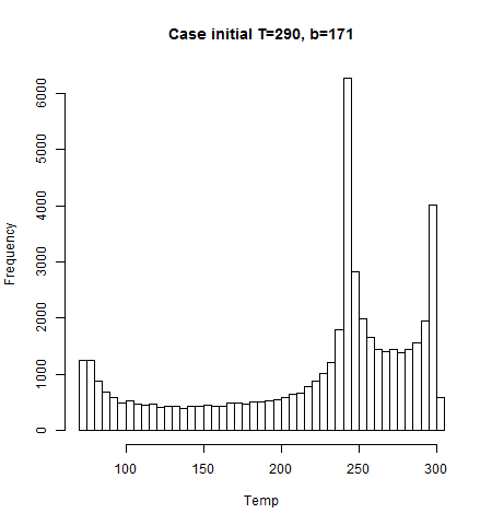
I'll demonstrate first how the individual runs, which give unpredictable results, give similar climate statistics. Then I'll talk more about what these statistics mean, and the mechanics of the chaos.As mentioned, the histogram of temperatures recorded has a characteristic pattern. Some bands are strongly favored. I'll explain why. But for now, here are two histograms, each of a run of 50000 steps starting from 300K (the second perturbed 300+1e-04), with b=170:
 |
 |
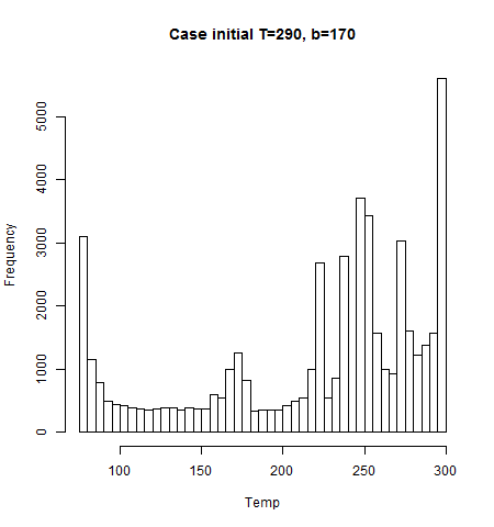
And here is a run starting from 290K. Again, very similar.
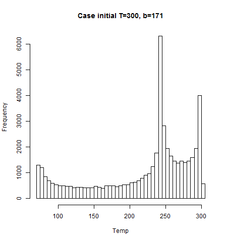
But if we change the parameter b from 170 to 171, the climate changes:
 |
 |
And the change can be measured again by the statistics of runs, each of which had no ability to predict individual time values.
Iterations and Chaos
The recurrence is of the formTn+1=F(Tn)+
where F takes the form
F(t)=T+b*(1-(T/Te)4)
I'll graph this function for various b:
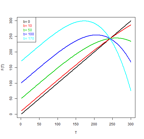
The curves all cross at E=(243,243). b=100, and b=170 are the parameters from the WUWT post, and b=170 is thye chaotic case done here.
The iteration process can be thought of as taking a T vlue, moving vertically to (T,F(T)), then horizontally to the diagonal line, as (F(T),F(T)). Then continue vertically to (F(T),F(F(T))), and so on. For small b, the curve is close to the diagonal, so the process moves in small steps to E. This is the proper process for solving the DE. For b large enough that the derivative at E is zero (b=60.75, the time constant t0 of the previous post), The first step goes almost immediately to E. For higher b, up to 2*t0, the path is a series of boxes, spiralling down to E. That includes b=100. But for b>2*t0, the boxes generally include E but do not converge. Here is one such case:
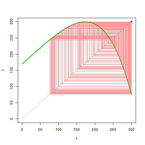
The maximum of F has a special role. It bounds the region of paths; no horizontal path can be lower, and if you follow a path from there, it goes to the furthest point that it can reach on the right, which then goes to the lowest reachable point. These are the bounds.
Two adjacent paths meeting the part of the curve on the right, will then bend to include a much larger width. That is the mechanism by which adjacent paths diverge, crating chaos. Conversely, meeting on the left, with low slopes, converges the paths. This is especially strong at the top. But the net result is divergence.
Here is a plot of the log of the distance between two paths which start out very close (0.0001).
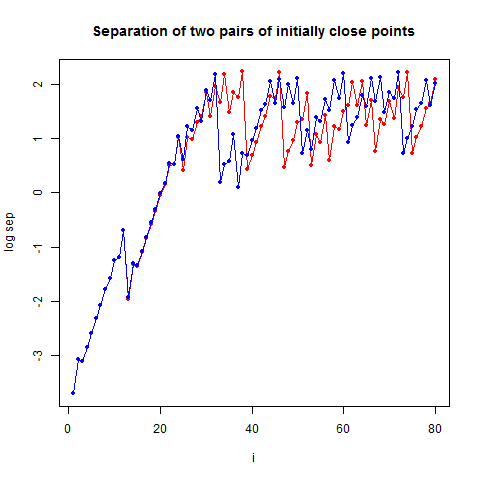
You'll see that it is initially linear (exponential increase), but that can't go on for ever. It is characterised by sudden drops. This happens when the two paths happen to come near the maximum of F. This is a broad region which is converted to a very narrow region. The distance drops and grows again gradually. But this contraction happens after the points have got all out of order, so it can't restore order.
I have an ambition to see an interactive chaos (well, it's Moyhu) which would show the paths in motion, with controllable parameters. Maybe for Xmas.


0 comments:
Post a Comment